plot,tt,f/nk
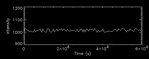
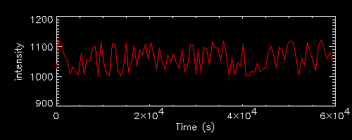
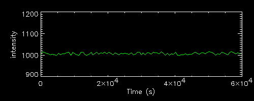
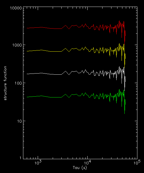 The colours correspond to the 4 light curves plotted on the left.
The SF scales exactly as the square of the fluctuations and is of course flat, pure white noise, so that one can reasonably compute its mean.
| plateau | level | factor | mean | sdev | mean SF | factor |
|---|---|---|---|---|---|---|
| 1000 | 15.81 | 1 | 1015.08 | 9.617 | 184.553 | 1 |
| 1000 | 31.62 | 2 | 1030.16 | 19.23 | 738.211 | 4 |
| 1000 | 63.25 | 4 | 1060.31 | 38.47 | 2952.84 | 16 |
| 1000 | 07.91 | 0.5 | 1007.54 | 4.808 | 46.1382 | 0.25 |
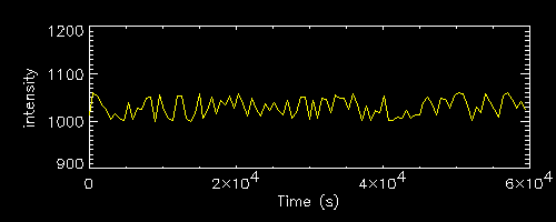
Let us then assess the effect of intensity generating uniform light curves with different plateau (1000 and 2000) and the same percentage level of fluctuations.
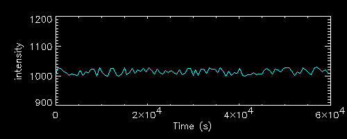
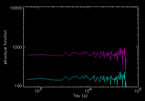 The colours correspond to the 2 light curves plotted on the left.
The SF scales this time exactly as the square of intensity
| plateau | level | factor | mean | sdev | mean SF | factor |
|---|---|---|---|---|---|---|
| 1000 | 30 | 1 | 1014.30 | 9.123 | 166.097 | 1 |
| 2000 | 60 | 2 | 2028.61 | 18.25 | 664.390 | 4 |
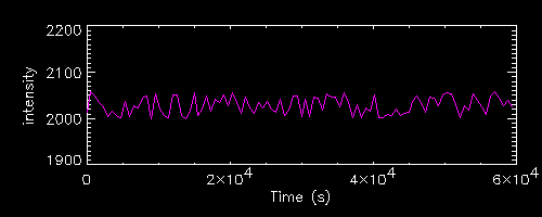
Let us then examine the SF of a periodic (sinusoidal) modulation, superimposed on the previous white noise light curve.
makesin,t,cc,100.,3230.
lcs=lc+cc
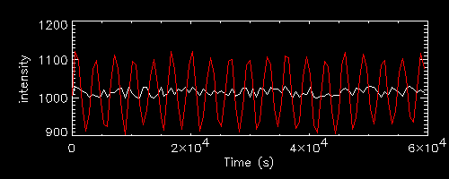
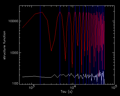
The SF of a periodically modulated white noise light curve (in red on the
right) is also periodic, with equal height maxima at P/2+nP and minima
tangent to the SF of the reference light curve
The blue vertical line indicates P/2+nP
The example shown is with a period reasonably large and not multiple of the bin size (600 s), i.e. not so well sampled. Tests have been made with other periods, with similar results (although for periods smaller than 600 s the periodicity is poorly determined, and for submultiples of 600 s (or 600 s itself) there is no contribution to the SF (the modulation adds to fixed bins).
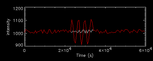
The next case is the addition to the reference white noise light curve of finite wavetrains derived from the same sinusoidal light curves (for a non-integer small number of periods)
lcs=lc
lcs(u)=lcs(u)+cc(u)
plot,tt,fs/nks
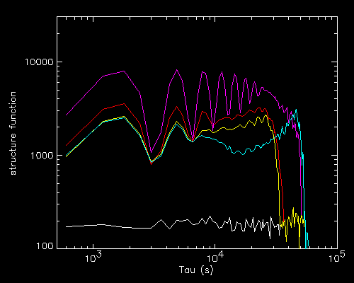
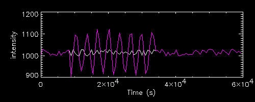
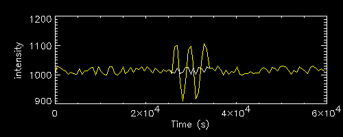
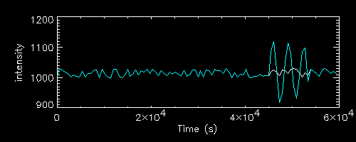
The colours correspond to the 4 light curves plotted on the left, while the white line is the SF of the reference light curve.
The first three light curves (red, magenta and yellow) are all wavetrains
ending at the same moment but covering a different number of cycles
(the number of peaks in the SF match the number of cycles).
The fourth light curve (cyan) is a wavetrain of the same duration
as the third (yellow) one, but located elsewhere.
All SF show similar features, that is, a number of peaks of decreasing amplitude (matching the number of cycles in the wavetrain) and a sharp drop which connects exactly with the reference light curve.
The location of the drop seems somewhat correlated with the duration of the wavetrain.
The cyan SF however is strange since the drop is very close to the end of
the tau axis, and there is an intermediate dip in the SF.
However one shall also note that the wavetrain in the cyan light curve is
located close to the end of the time interval covered, and anyhow well past
its middle. The simplest examples of single flares shown below could help
to understand the shape of the fourth SF.
Since sinusoidal variations are quite unlikely in the sources we are interested in, a simpler example superimposes onto the white noise light curve a single flare derived from the positive part of a single sinusoidal cycle (with the period and resolution chosen this is just less than 4 time bins).
lcs=lc
lcs(i+3)=lcs(i+3)+flare
plot,tt,fs/nks
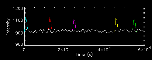
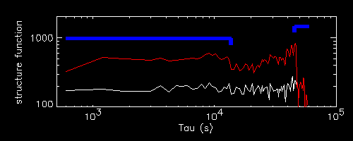
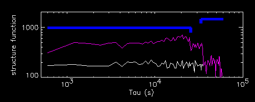
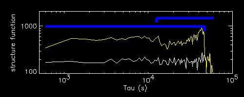
The colours correspond to the 5 SF plotted on the right, while the white line is the reference light curve (or its SF). Each analysed light curve differs from the reference only in the single flare highlighted in colour.
Each flare is located at bin i and lasts 4 bins (the last one is forced to
be zero, i.e. equal to the reference curve, instead of the negative value
in the original sinusoid, compare IDL expression above), i.e. 1800 s.
The range of time bins interested by the flares is printed above each SF.
The two blue L-shaped lines in the SF plots extend respectively :
- from the left end of the tau range to the end time of the flare tend=t(i+3)
- from the right end of the tau range (lastt) back to lastt-tend
The features of the SF can be described as follows :
For the first two light curves (red and magenta), which correspond to flares located in the first half of the light curve, the SF shows a shallow peak, followed by a little drop in correspondence of tend, followed by a plateau or shallow dip, followed by a sharp drop in correspondence of lastt-tend after which one reaches exactly the reference SF.
For a flare located in the second half of the light curve (like the third, in
yellow) the location of the two drops (the minor one and the sharp one) is
reversed. The terminal, sharpest drop corresoponds to the end time of the
flare tend
This is true, although less legible, also for a flare located close to the end
of the light curve (like the fifth, in green, SF not shown)
A flare located at the very beginning of the light curve (fourth, in cyan)
shows a steady rise without final drop, and also the minor drop at tend
is almost invisible.
A flare located at the very end of the light curve (not shown) gives a SF
at all similar.
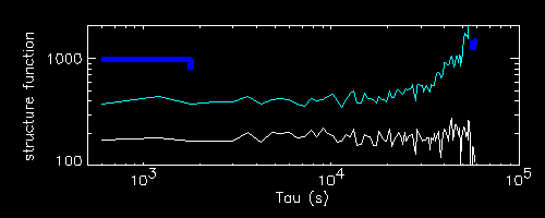
Let us examine the effect of the intensity of a single flare.
The red curve is the same reported above for a flare at i=20 (12000-13800 s), while the green curve corresponds to a flare of double intensity occurring at the same time.
One can see that the two SF have approximately the same shape, with the same features at the same positions, but with the one corresponding to the more intense flare being scaled up.
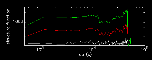
Let us examine the effect of multiple flares.
The red and magenta curves are the same reported above for a flare at i=20 and i=40, while the green curve corresponds to a light curve with two flares of the same intensity occurring at both i=20 and i=40.
One can see that the green SF stays up until the time of the drop of the red curve (end of first flare) where it has a dip. then stays up again mimicking the magenta curve until the time of the final drop of the magenta curve : at this point it drops until it superimposes exactly to the red curve, which then follows until the red (hidden) and green drop together to the reference white noise value.
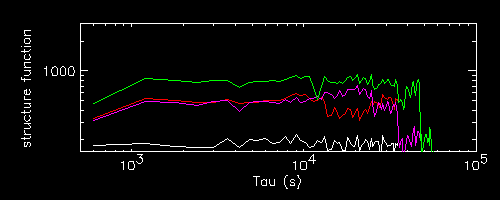
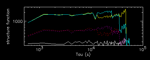
One can see that the main features occur as sharp drops at characteristics times, connecting otherwise almost flat portions of the SF curve.
I suspended writing these pages on Oct 15. I restart now on Oct 30 adding some results obtained 2 weeks ago and not yet inserted here.
Let us examine now the behaviour of red noise (or something similar to it), which I generate co-adding several sinusoids of different periods and amplitude proportional to a power of period using the following IDL code :
lcc1=lcr1-lcr1+1000
seed=123456789L
for i=P1,P2 do begin
makesin,t+randomu(seed)*i,cc,float(i),float(i)
lcr1=lcr1+cc/(P2-P1)
endfor
seed=123456789L
for i=P1,P2 do begin
makesin,t+randomu(seed)*i,cc,float(i),float(i)
lcc1=lcc1+cc/(P2-P1)
endfor
use a flat light curve at intensity 1000 as base for the "c" light curve
assign a random seed
loop from period P1 to period P2
generate a sinusoid of amplitude proportional to period
and co-add it to the "r" light curve, normalize by number of periods used
reassign same random seed to have same noise
loop from period P1 to period P2
generate same sinusoid as above
and co-add it to the "c" light curve, normalize by number of periods used
The "r" light curve is the superposition of white noise with red noise from P1 to P2, while the "c" light curve should be pure red noise.
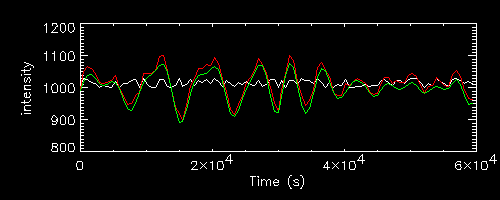
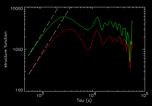
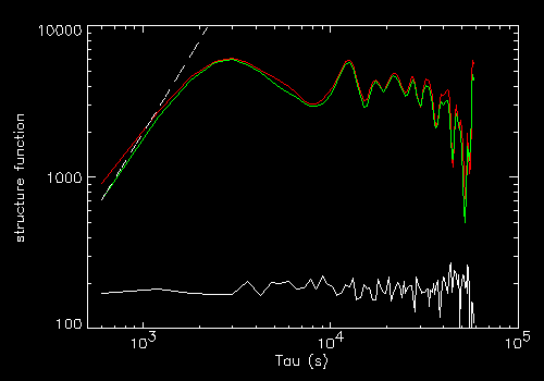
"r" (red) and "c" (green) light curves for P1=3000, P2=10000 s
On the right their SF compared with the white noise one (in white).
The dashed line is a tau2 power law normalized to the first point.
Since the "c" curves are very similar to the "r" curves, just smoother, we
limit ourselves to the pure red noise "c" curves in what follows.
One can note that the SF of the "c" curve is smoother, and closer to the
tau2 slope in its beginning.
The other feature is that the first peak is at P1, and ends approximately
before P2
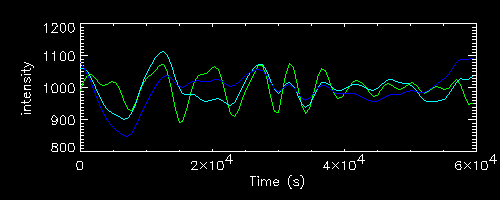
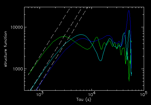
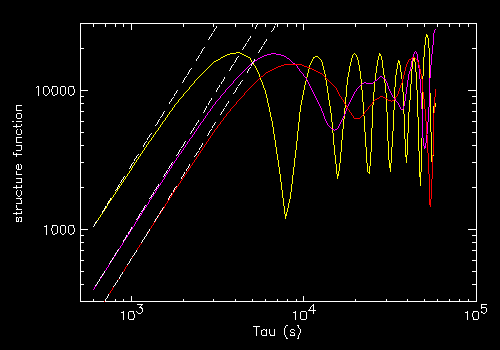
"c" red noise light curves for the following period ranges (same start)
- P1=3000, P2=10000 (green, same as above)
- P1=3000, P2=20000 (cyan)
- P1=3000, P2=30000 (blue)
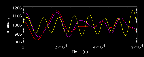
"c" red noise light curves for the following period ranges (another start,
but same ends as the previous family)
- P1=7000, P2=10000 (yellow, compare with green above)
- P1=7000, P2=20000 (magenta, compare with cyan)
- P1=7000, P2=30000 (red, compare with blue)
On the right their SF with the respective tau2 (dashed) trends
which is confirmed.
However the relationship between the location of the peak and the range P1-P2
where the noise is defined is unclear.
The situation is even more complex when P2 is 30000 s, i.e. half of the total
interval.
I am however not sure at all that the "red noise" simulations are by any mean realistic (but a periodic function is simpler than shot noise).
makesin,t+randomu(seed)*i,cc,1.E-4*float(i)^2,float(i)
The red curve below has been generated with such formula in the period range i=P1,P2 with P1=3000 and P2=10000 (same as the reference green curve, which has been generated with the default formula (amplitude proportional to period).
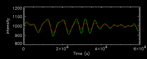
The relevant SFs are reported on the right. They scale in a similar way, with just minor shifts of the peak, and the initial rise in both cases follows a tau2 trend (despite the different power index used in the simulation)
