Benchmarks revisited

Twenty years after

Lucio Chiappetti - INAF IASF Milano05 Feb 2009

Cosi' per li gran savi si confessa
che la fenice muore e poi rinasce
quando al cinquecentesimo anno appressa

Inf. XXIV,106-108

Introduction

Principles

Introduction

After almost 19 years since the time I wrote the first version of the report "R15" "A set of simple benchmark programs for representative cases in X-ray astronomy", I am revisiting my benchmarks, which compare the relative speed of some realistic programs on different platforms and operating systems, to look at progress in computing speed over such period of time, and to see where we stand now.

The quoted document was last updated in 1993, however the benchmarks were ran again in 1998, 2000 and 2005 without formal documentation of the results. I try to recover such material as well.

I am therefore presenting here a partial, but formal, update.
This benchmarks have no pretense of an extremely objective measurement of the relative performance of machines or compilers, but should give an idea of what one can expect in cases drawn from real life programs.

Principles

The original benchmarks included two main programs plus a support program (all written in Fortran) and two support files. They are presently accessible here :

benchdft	Representative benchmark, direct Fourier transform
benchmat	Support program for the next benchmark
matrix.ascii	Support file, to be converted in binary form running benchmat, the output file used for the next benchmark
spectrum.test	Support file used for the next benchmark
benchfit	Representative benchmark, X-ray spectral fitting
benchfit	Patched version for Linux g77 (see below)

For details on their usage refer to report R15
The benchdft benchmark can be run with different input parameters, i.e. the number of data points, and the number of frequency steps. The time should scale lineary with either parameter.
The benchfit benchmark instead can be run in a single condition and performs a fit on canned data using canned initial guesses.
Both benchmarks shall be repeated a few times, ideally on an unloaded machine, and the fastest execution times shall be noted down.

The programs can be compiled with different compilers, and with different optimization levels.

Caveat ! The original version of benchfit does not compile on Linux using g77, because such compiler is very picky and the program has a routine with two entry points (of which one is a FUNCTION and the other a SUBROUTINE). A patched version of the code is provided. Such version compiles, however the executable generated by g77 does not run correctly (the fitting procedure enters an infinite loop). I have not investigated the matter, but instead moved to the use of other compilers. In general the mixing of FUNCTION and SUBROUTINE entries is accepted by them, with or without warnings.

Updated results

In the following I summarize graphically the results of a number of tests performed either in the past, or at the time of writing. Namely:

The tests on IBM VM/SP, HP RTE, VAX VMS, early Sun 4 workstations with SunOS, and DECstation Ultrix are taken from report R15. Such report contains also some results derived on Windows PCs which are not used here.
The tests on Sun Sparc workstations with Solaris, DEC Alpha workstations with OSF aka DU aka Tru64, and HP-UX were run in 1998 and 2000. They were run systematically on a number of machines, but I'm not reporting results for all the Sparc w/s but just for a selection. I found a paper-only note, so I am now able to reconstruct the make and model of the individual Sparc.
A single test was run in 2005 comparing the DEC Alpha (test repeated) with a single Linux w/s whose make and model was not recorded. The test was done using g77, i.e. refers only to benchdft.
The remaining tests on Linux were run in 2009 and, with one exception using g77, refer to the Intel ifort compiler.
I have chosen one machine out of each of the main groups we have with the same model, plus two standalone but faster machines.

The benchmark programs return a number of execution times of their different steps, as detailed in report R15. De facto, most of such times (i/o or data generation) are irrelevant for our purposes. The relevant times to measure CPU consumption are the time for fitting in benchfit and the time for the Fourier transform in benchdft. For our purposes we use as reference for the latter a run with 10000 data points and 100 frequency steps.
The fitting and Fourier transform times (T_fit and T_Four) do not scale always exactly in the same way (due to the different nature of the algorithm), and in particular sometimes scale differently with different optimization levels.

In order to provide a summary, one shall compare a given measure with the equivalent measure of a reference machine (and OS and optimization). R15 used an IBM VM/SP system as reference, which nowadays is completely out of date. In 1998-2000 the reference used was my DEC Alpha 255, and for simplicity in re-use of the old measures I continue to use such reference.
In principle one can normalize any measure, e.g. R_fit=T_fit/T_fit(ref) etc. In practice I decided to take the mean of R_fit and R_Four (for the 10000/100 case), and the associated standard deviation as error bar.
In practice

The reference times for the DEC Alpha 255 measured in 2005 were recorded in a file
For the measurements done within 1993, the full details of individual measurements are contained in R15
For the measurements done in 1998 and 2000, I thought the individual measurements were no longer available. A file recorded only a relative mean with error bar. I was not sure whether such mean included only R_fit and R_Four for a single optimization levels, or also different levels or additional measurements. I retro-fitted R_fit and R_Four assuming they were the only elements in the mean, and the results are not inconsistent.
However I later discovered a paper note with the individual results, so I updated the database with them.
For the recent results I have all details, some of which are reported below.
I inserted all available information in a database, which is available privately, but report here only the mean and error.

These are the recent results. All times are in seconds. The mean and error are relative to the reference (entry in red) measured in 2005. As said above, g77 does not allow to run benchfit. The bulk of the tests have been done compiling with an oldish Intel compiler 8.1 on poseidon, using options save i-static and running the compiled executables also on the other machines. The default optimization level is -O2. Since there are no speed changes already after -O1, -O3 was not tested.

Machine	Model	Compiler	benchdft					benchfit	average
Machine	Model	and option	DG 100	DF 100	DG 10000	DF 100	DF 500	CURFT	mean	error
poseidon III	DEC Alpha 255	native	0.001	0.016	0.015	1.355	6.752	0.796	1.0	n/a
poseidon IV	HP dc7100	g77	0.000	0.002	0.002	0.220	1.089	n/a	0.160	n/a
poseidon IV	HP dc7100	ifort -O0	0.000	0.000	0.000	0.140	0.700	0.100	0.114	0.015
poseidon IV	HP dc7100	ifort -O1	0.000	0.000	0.000	0.130	0.650	0.040	0.073	0.032
poseidon IV	HP dc7100	ifort -O2	0.000	0.000	0.000	0.130	0.650	0.040	0.073	0.032
obelix	custom	ifort -O2	0.000	0.000	0.000	0.070	0.370	0.030	0.044	0.010
metis	custom	ifort -O2	0.000	0.000	0.000	0.140	0.730	0.070	0.095	0.011
antigone	Dell GX620N	ifort -O2	0.000	0.000	0.000	0.120	0.630	0.040	0.069	0.027
cora	HP dx2400	ifort -O2	0.000	0.000	0.000	0.110	0.400	0.060	0.078	0.004
galileo	Dell T7400	ifort -O2	0.000	0.000	0.000	0.050	0.290	0.020	0.031	0.008

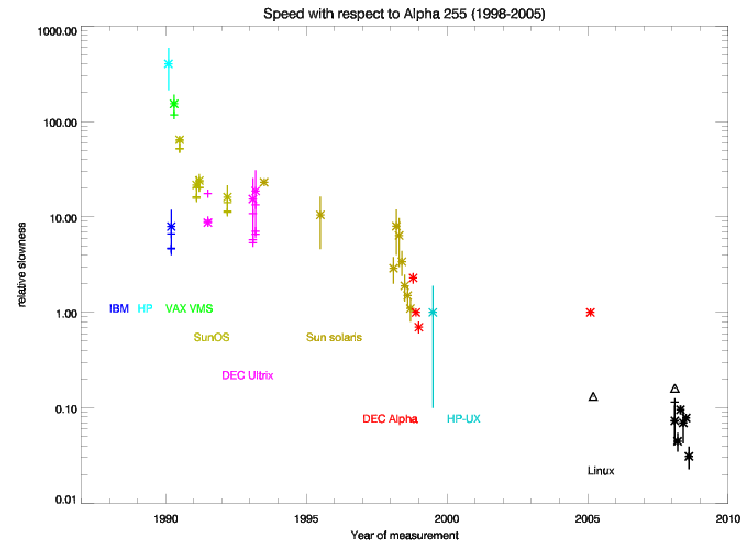
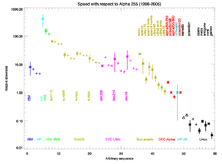
And here are some graphical summaries of the average values for the entire dataset.
The first figure reports the relative speed as a function of time (the time is not the time a machine was acquired, nor the actual time of measurements : measurements are grouped by year according to the content of R15 or later runs, and then displaced arbitrarily inside the year).
For each machine, one value is chosen as representative for the mean and error bar, and indicated with an asterisk. This is usually the compilation without optimization, except for Linux where it is the default (ifort -O2). Where tests with different optimization levels were run, they are indicated with crosses (no error bars). Triangle mark the tests with g77.
The reference measurement (relative speed = 1) is reported twice (1998 and 2005)

The second figure reports the same data in arbitrary order of occurrence (which coincides with the chronological order of the previous figure, but allows a clearer expansion). The representative value (asterisk) is labelled with the machine model (for data taken from R15 or 2000 paper note) or the machine name (for later data). Measurements with other optimization levels (crosses) are reported unlabelled on the right of the representative one.

Cross language tests

In addition to the traditional "revisited" benchmarks, I decided to test the capabilities of different languages and/or compilers. I therefore concentrated on the Direct Fourier Transform benchmark, which is rather easy to convert across languages, and willingly a more intensive algorithm than other more efficient equivalent ones (e.g. FFT). I hence developed the following versions :

benchdft.f is the standard Fortran benchmark, which was tested under g77, ifort, g95 and gfortran.
benchdft.pro is an IDL version, which can be invoked as
benchdft npoints nfrequencies
It was tested under IDL 7.0.
benchdft.c is a C version, which can be compiled as
cc benchdft.c -lm -On -o cbench
and invoked as
cbench npoints nfrequencies.
It was tested with gcc 3.3.4.
benchdft.java is a Java version, which can be compiled as
javac benchdft.javac
and invoked as
java benchdft npoints nfrequencies.
It was tested with javac 1.6.0_10.

No particular care has been given to numerical accuracy issues, although the results are not inconsistent with respect to the Fortran ones.
All tests were run on the same machine (mine, poseidon) with the exception of the gfortran test (see below).

The IDL version has not been recoded in optimal way (some DO loops have been recoded as array assignments, but the main loop in subroutine DCDTF has not been recoded. It uses a native call to compute the processing time.
The procedure allocates memory dynamically, however shows no paging effect since the linear scaling in both directions is preserved. Also excluding the allocation of the work arrays in the subroutine from the time count shows no change in the times.

The C version requires the mathematical library. Memory is allocated statically, and all the work arrays are global to avoid issues with passing arguments (something I've never been very good in C). The code includes a routine to measure processing time which I adapted from something I had (and did not write myself), which I hope makes sense.
I tested it with the default optimization (i.e. none) and also with -O1 and -O2. There is a marginal improvement going to -O1 and nothing going to -O2.

The Java version uses global work arrays to avoid issues with passing arguments, but memory is allocated in the subroutine method. It uses a native call to compute the processing time. I had to use the Math.IEEEremainder call (not the "%" operator) for modulo inside the main loop, if I wanted to obtain results numerically consistent with the Fortran ones.

I have also run two tests using other (free) Fortran compilers.

One test was run using the g95 compiler, using the default optimization (-O1; using -O2 should make things run faster, i.e. in 93% of the time). Binary version g95 0.91 (G95 Fortran 95 version 4.0.3 aka gcc version 4.0.3).

Another test was run using the gfortran compiler. However due to an incompatibility at glibc level, I could not install gfortran on my workstation, therefore I installed in a scratch area GNU Fortran (GCC) 4.4.0 on obelix (x86_64) and run the tests there. I also ran an ifort test on obelix to allow a cross calibration. The default is no optimization. Going to -O1 nearly halves the times (factor 0.62), while -O2 is the same as -O1.

The numeric results are reported here below. All times are in seconds. The values for gfortran (in italics) are reconstructed values, rescaled to poseidon from the original obelix measure assuming it is 2.39 times slower than obelix where they were measured at -O2.

N.Freq.steps	100							500							1000
N.points	ifort	g77	g95	gfortran	gcc	java	IDL	ifort	g77	g95	gfortran	gcc	java	IDL	ifort	g77	g95	gfortran	gcc	java	IDL
100	0.000	0.003	0.003	0.009	0.000	0.021	0.051	0.000	0.017	0.014	0.009	0.020	0.081	0.248	0.010	0.031	0.030	0.038	0.030	0.121	0.493
1000	0.010	0.031	0.030	0.019	0.030	0.139	0.480	0.080	0.155	0.143	0.086	0.150	0.574	2.393	0.160	0.307	0.284	0.163	0.300	1.125	4.796
5000	0.080	0.156	0.145	0.076	0.150	0.614	2.368	0.410	0.769	0.715	0.393	0.740	2.943	11.957	0.830	1.535	1.427	0.786	1.470	5.893	24.100
10000	0.170	0.312	0.289	0.172	0.300	1.231	4.852	0.840	1.538	1.430	0.795	1.480	6.008	24.358	1.660	3.069	2.857	1.582	2.930	11.942	48.094

A graphical representation of the above is not particularly useful, and simply shows what is already apparent from the table, i.e. that the time scales linearly with the number of data points or frequency steps, with the possible exception of the cases for very small numbers of points or steps which are presumably poorly defined, or affected by some constant overhead. If such values are excluded, one can summarize as :

gfortran (-O2) is estimated 1.09 times slower than ifort
gcc is 1.61 times slower than ifort
g95 is 1.74 times slower than ifort
g77 is 1.88 times slower than ifort
java is 7.2 times slower than ifort
IDL is 29.3 times slower than ifort

Of course each language has its own merits to be used for particular applications, so the above figures should not be used beyond their face value.

sax.iasf-milano.inaf.it/~lucio/bench/ :: original creation 2009 feb 05 18:36:05 CET :: last edit 2009 Feb 05 18:36:05 CET

Cosi' per li gran savi si confessa che la fenice muore e poi rinasce quando al cinquecentesimo anno appressa
Inf. XXIV,106-108